Regularization
Learning Objectives
- Regularization (L2)
- Capacity Control
- Regularization for linear and logistic regression
Regularization
Intuition of regularization
Known :
- If $\mathcal{H}$ to complex: most probable overfitting.
- Polynominals with high degree have higher model complexity as polynominals with lower degree.
Polynom of grade 4: $$ h_\theta(x) = \theta_0 + \theta_1 x + \theta_2 x^2 + \theta_3 x^3 + \theta_4 x^4 $$
Constraint $\theta_3 = \theta_4 = 0$ should lower the model complexity.
Constraint: $|\theta_3| \leq \epsilon$ and $|\theta_4| \leq \epsilon$ with small $\epsilon$ $\rightarrow$ model complexity should only has increased a little bit.
Cost function for regularization
Cost funktion for polynom of degree 4 with constraint: small values for $\theta_3$ and $\theta_4$:
$$ J(\theta) = \frac{1}{2m} \sum_{i=1}^{m} (h_\theta(x^{(i)}) - y^{(i)})^2 + \lambda \theta_3^2 + \lambda \theta_4^2 $$
with large hyperparameter $\lambda$.
Regularization for linear regression
- Small values for $\theta_0, \theta_1, \ldots, \theta_n$ result in ``simpler'' hypotheses $\rightarrow$ less overfitting
- Many features ( e.g. example "housing prices")
$\rightarrow$ same features have less or no information $\rightarrow$ bad generalization.
Regularization on $\theta$-values suppresses such feature.
Cost function with regularization
\begin{align*} J(\theta) = &\frac{1}{m} \left[ \sum_{i=1}^{m} loss(h_\theta(x^{(i)}),y^{(i)}) + \frac{\lambda}{2} \sum_{j=1}^n \theta_j^2 \right] %// = & \frac{1}{2m} \left[ \sum_{i=1}^{m} loss(h_\theta(x^{(i)}),y^{(i)}) %+ \frac{\lambda}{2} \vec \theta^T \vec \theta \right] \end{align*} with
- $\lambda$: regularization hyperparameter - controlls the complexity of the model.
- large $\lambda$ $\rightarrow$ low complexity
- small $\lambda$ $\rightarrow$ high complexity
- typically: no regularization of $\theta_0$
Augmented Error
Instead of minimization of $J_{train}$ (training error) we minimize an augmented error}: $$ J_{aug} = J_{train}(\theta) + \frac{\lambda}{m}\Omega(\theta) = J_{train}(\theta) + overfit penalty $$
Recap: gradient descent
Cost function $$ J(\theta) = \frac{1}{m} \left[ \sum_{i=1}^{m} loss(h_\theta(x^{(i)}), y^{(i)}) + \frac{\lambda}{2} \sum_{j=1}^n \theta_j^2 \right] $$
with the Update Rule
$$ \theta_j \leftarrow \theta_j - \alpha \frac{\partial}{\partial \theta_j} J(\theta) $$
gradient descent with regularization for the linar and logistic regression
for $j=0$ (no change) $$ \theta_j \leftarrow \theta_j - \alpha \frac{1}{m} \sum_{i=1}^m (h_\theta(\vec x^{(i)}) - y^{(i)}) x_0^{(i)} $$ for $j \neq 0$ $$ \theta_j \leftarrow \theta_j - \alpha \left[ \frac{1}{m} \sum_{i=1}^m (h_\theta(x^{(i)}) - y^{(i)}) x_j^{(i)} + \frac{\lambda}{m} \theta_j \right] $$
Interpretation: Weight Decay
Transformation of the update rule for $j \neq 0$ results in $$ \theta_j \leftarrow \theta_j (1-\alpha \frac{\lambda}{m}) - \frac{\alpha}{m} \sum_{i=1}^m (h_\theta(\vec x^{(i)}) - y^{(i)}) x_j^{(i)} $$
In comparision with the update rule without regularization we see that $\theta_j$ is multiplied with an weight decay factor: $$ (1-\alpha \frac{\lambda}{m}) < 1 $$
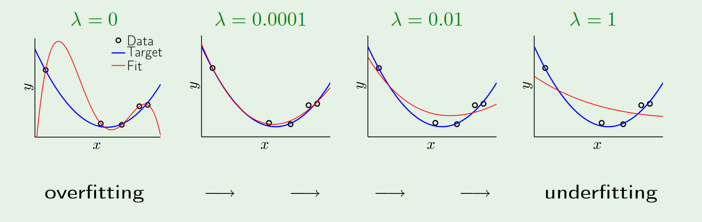 (from [Abu])
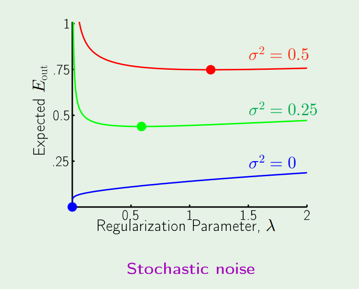
$\lambda$ and noise
 (from [Abu])
Performance of the uniform regularizer at differnt levels of stochastic noise $\sigma$. Both target and model are polynominals of order 15.
Exercise
Extend your "linear and logistic regression" implementation with regularization.
- Extend the
get_cost_function(loss, lambda_reg) - Extend "gradient descent" and learn a logistic regression model with regularization.
- For debugging: Plot the progress (cost value over iterations)
- How does the theta values differ from the unregularized logistic regression? Is there a change in the decision boundary? Is there a difference in the prediction of the class probabilities?
Literature:
- [Abu] Yaser Abu-Mostafa
- Learning from Data, Caltech Machine Learning
- Learning from Data, AMLBook 2012
- Andrew Ng: Machine Learning. Openclassroom Stanford University, 2013
- [Has] Trevor Hastie,Robert Tibshirani, Jerome Friedman: The Elements of Statistical Learning, Chaper 7, Springer Verlag 2009