Multivariate Linear Regression
Learning Objectives
- Multivariate linear regression
- Vector implementation
- Input Scaling
- Concepts of machine learning: learning, cost function, gradient descent
- Basis functions
Problem formulation
Supervised learning: regression
- $m$ observations (training examples) with
- $n$ Features:
- $i$-th training example
- ${\bf x}^{(i)}= \{ x_1^{(i)}, x_2^{(i)}, \dots, x_n^{(i)}\}$
- $x_j^{(i)}$: value of the feature $j$ for the $i$-th example
- $1 \leq j \leq n$ (univariate case $n=1$):
- $i$-th target value $y^{(i)}$
- $i$-th training example
Goal: prediction of $y$ for a new $\bf x$.
Example Boston data
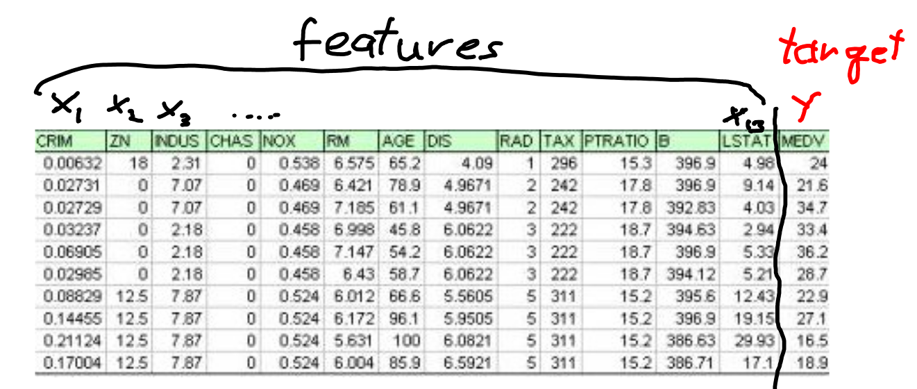
Boston feature names
#load data
from sklearn.datasets import load_boston
boston = load_boston()

# feature names
#boston.feature_names
# features (vec x)
#print(boston.data)
# house price (y)
#print(boston.target)
Linear model
- linear with respect to the parameters $\theta_j$
- (for now) linear with repect to $x_j$
print (boston.DESCR)

# feature names
print(boston.feature_names)

# features (vec x)
print(boston.data)

# house price (y)
print(boston.target)
Vector formulation
Hypothesis: $h_{\theta}(\vec{x}) = \vec{\theta}^T \cdot \vec{x} = \theta_0 x_0 + \theta_1 x_1 + \dots \theta_n x_n $
- with $x_0 = 1$
- $n+1$ parameter: ${\vec{\theta}}^T = ( \theta_0, \theta_1, \dots , \theta_n ) $
for convenience we use $\theta$ as symbol for all $\{ \theta_0, \theta_1, \dots \}$
Cost function and gradient descent
Minimization of the cost function $J$
$$ J({\theta}) = \frac{1}{2 m} \sum_{i=1}^m (h_{\theta}(\vec{x}^{(i)}) - y^{(i)})^2 $$Recap: Gradient Descent
Repeat until convergence:
$$ \theta_j \leftarrow \theta_j - \alpha \frac{\partial}{\partial \theta_j} J(\theta) $$Vector form of the update rule
with the definition of the gradient $$ grad(J(\theta)) = \vec \nabla J(\theta) = \left( \begin{array}{c} \frac{\partial J(\theta)}{\partial \theta_0} \\ \frac{\partial J(\theta)}{\partial \theta_1} \\ \dots \\ \frac{\partial J(\theta)}{\partial \theta_n} \end{array}\right) $$
$$ \vec \theta^{neu} \leftarrow \vec \theta^{alt} - \alpha \cdot grad(J(\theta^{alt})) $$
Partial derivates for linear regression
\begin{align*} \frac{\partial}{\partial \theta_j} J(\theta) &= \frac{\partial}{\partial \theta_j} \frac{1}{2m} \sum_{i=1}^m (h_\theta(\vec x^{(i)}) - y^{(i)})^2 \\ & = \frac{\partial}{\partial \theta_j} \frac{1}{2m} \sum_{i=1}^m (\vec \theta^T \cdot \vec x^{(i)} - y^{(i)}) ^2 \end{align*}So we have update rules for all $\theta_j$ ($0 \leq j \leq n$):
$$ \theta_j \leftarrow \theta_j - \alpha \frac{1}{m} \sum_{i=1}^m (\vec \theta^T \cdot \vec x^{(i)} - y^{(i)}) x_j^{(i)\ } $$Vector form of the update rule for linear regression
$$ \vec \theta^{new} \leftarrow \vec \theta^{old} - \alpha \frac{1}{m} \sum_{i=1}^m (\vec \theta^T \cdot \vec x^{(i)} - \ y^{(i)}) \vec{x}^{(i)} $$Feature Scaling
If the features have different order of magnitude: the learning will be very slow (see e.g. here on pages 26-30).
A remedy is rescaling of the features.
Idea: values of all {\it Features $x_j$) should be in the range: $$ -1 \lesssim x_j \lesssim 1 $$
Z-transformation
$$ x_j' = \frac{x_j-\mu_j}{std(x_j)} $$with
- mean of $x_j$: $\mu_j = \overline{x_j}= \sum_i x_j^{(i)} / m $
- standard deviation of $x_j$: $std(x_j) = \sqrt{var(x_j)}$
- variance of $x_j$: $var(x_j) = \overline{(x_j - \mu_j)^2} = \overline{x_j^2} - \mu_j^2$
For all features $x_j'$ the mean is 0 and the standard deviation is 1.
Implementation and practice
Data matrix (design matrix)
Train data as matrix ${\bf X}$ with $X_{ij} \equiv x_j^{(i)}$
- each rows $i$ corresponds to a training example $\vec x^{(i)}$
- each column $j$ corresponds to the $j$-th feature
- with $x_0^{(i)} = 1$
Prediction can be done for all data by:
$$\vec{h}({\bf X}) = {\bf X} \cdot \vec{\theta}$$import numpy as np
# dummy values
X = np.random.randn(700,4)
theta = np.array([2.,3.,4.,5.])
# e.g.: with 3 features and 700 training data with numpy:
print (X.shape)
print (theta.shape)
h = X.dot(theta)
print (h.shape)
Vectorisierte Form of the update rule with Data Matrix $\bf X$
From the vectorised form of the update rule
$$ \vec \Theta^{new} \leftarrow \vec \Theta^{old} - \alpha \frac{1}{m} \sum_{i=1}^m (h(\vec x^{(i)}) - y^{(i)}) \vec{x}^\ {(i)} $$we get with the data matrix ${\bf X}$ $$ \vec \Theta^{new} \leftarrow \vec \Theta^{old} - \alpha \frac{1}{m} {\bf X^T} \cdot ( \vec{h}({\bf X}) - \vec y) $$
in numpy:
theta = theta - alpha * (1.0 / m) * X.T.dot(h - y)For testing if the gradient descent implementation works
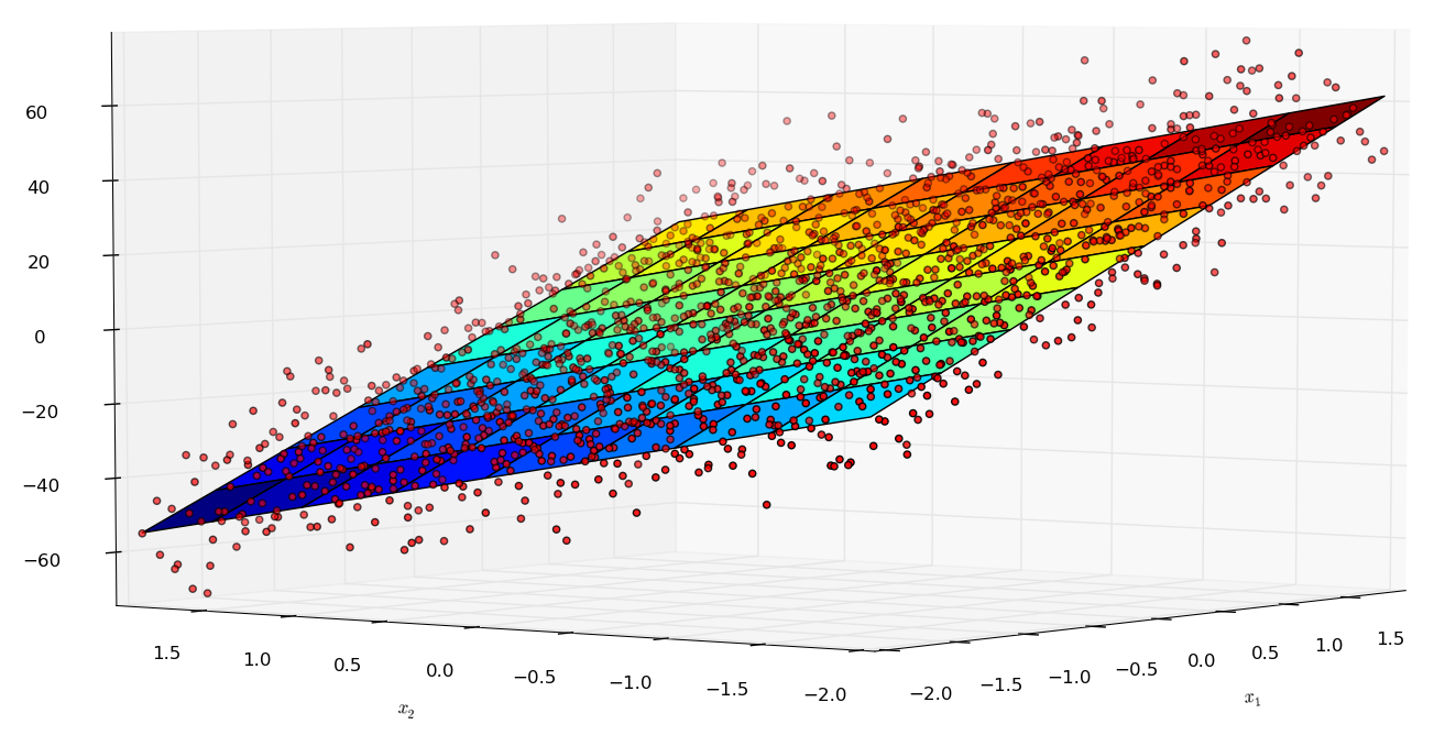
Remember the goal is to find the $\text{min}_\theta J(\theta)$
Plot $J(\theta)$ over the iterations: $J(\theta)$ must become smaller in each iteration (for full batch learning).
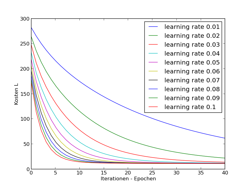
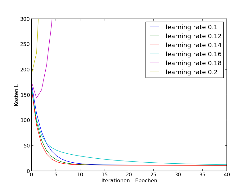
Learning Rate $\alpha$
How to choose $\alpha$?
Look at the progress during learning for different values of $\alpha$!
to small values for $\alpha$:
to large values for $\alpha$:
If $\alpha$ is to small $\Rightarrow$ smale convergence.
If $\alpha$ is to large $\Rightarrow$ $J$ grows or (oscillation or suboptimal progress). Wenn α zu groÿ ist, eventuell keine Konvergenz:
Try different $\alpha$'s (on log-space) or e.g.: 0.003, 0.006, 0.009, 0.03, 0.06, 0.09, $\dots$
Note: With feature scaling learning yield modified parameters : $\theta_0'$ und $\theta_1'$
\begin{align*} h(x) & = {\theta_0}' +{\theta_1}' x' \\ & = {\theta_0}' +{\theta_1}' \cdot \frac{x - \mu}{\sigma_x} \\ & = ({\theta_0}' - {\theta_1}' \cdot \frac{\mu}{\sigma_x} )+ \frac{{\theta_1}'}{\sigma_x} \cdot x \end{align*}i.e. \begin{align} \theta_0 & = \Theta_0' - \theta_1' \cdot \frac{\mu}{\sigma_x} \ \theta_1 & = \frac{\theta_1'}{\sigma_x} \end{align}
Basis functions
So far: The model is linear in respect to the input:
$$ h_\theta ({\vec x}) = \theta_0 + \sum_{j=1}^n \theta_j x_j $$Extension: Replace the $x_j$ with basis functions $\phi_k ( {\vec x}) $:
$$ h_\theta (\vec x) = \theta_0 + \sum_{k=1}^{n'} \theta_k \phi_k ( {\vec x}) $$Still a linear model. It's linear with respect to the parameters $\theta_j$
Examples for basis functions
Polynoms: $$ \phi_k ( {\vec x}) = x_1^2 $$
$$ \phi_{k'} ( {\vec x}) = x_1 \cdot x_3 $$``Gaussian Basis Functions''
$$ \phi_{k''} ( {\vec x}) = \exp\{ - \frac{(x-\mu_j)^2}{2 \sigma_j^2}\} $$(New) Features
- Transformation of the raw data $\vec{x_i}$ to features $\vec \phi(\vec x_i)$
Example: prediction of the price of land:
raw data: length $x_1$ and width $x_2$. \
instead: $h_\theta = \theta_0 + \theta_1 \cdot length + \theta_2 \cdot width $ \ \vspace{1cm}
use the ``area'' as feature $\phi_1$: $area = length \cdot width$
$$h'_\theta = \theta_0' + \theta_1' \cdot area $$
Polynominal regression
Exercise: Vector implementation of gradient descent
Note:
- The implementation should work with an arbitrary number of features.
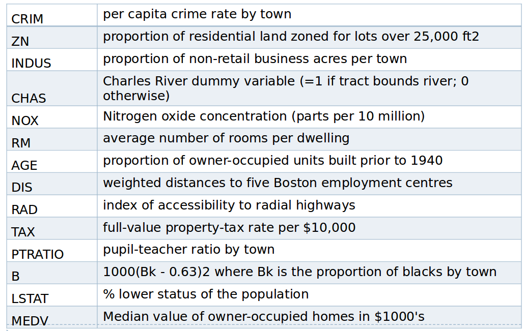
- Generate artificial data for the design matrix $\bf X$ with two features $x_1, x_2$ (or three with fixed $x_0=1$)
- Implement a
get_linear_hypothesisfunction:>theta = np.array([1.1, 2.0, -.9]) > h = get_linear_hypothesis(theta) > print (h(X)) array([ -0.99896965, 20.71147926, ... - Target values:
- Use the
get_linear_hypothesisfunction for generating y-values (add gaussian noise) - Plot the x1-x2-y data points in a 3D-plot, see http://matplotlib.org/mpl_toolkits/mplot3d/tutorial.html
- Use the
Implement the 'get_cost_function(x, y)' python function:
> j = get_cost_function(X, y)
> print (j(theta))
> 401.20  # depends on X and y
Implement gradient descent.
Implement a function for the update rule:
> theta = compute_new_theta(x, y, theta, alpha)Implement a function
gradient_descent(alpha, theta, X, y).thetaare the start values for $\vec \theta$. The function applies iterativelycompute_new_theta. Use an arbitrary stoping criterion.
Plot the progress (cost value over iterations) für 5B
Plot the optimal hypothesis in a graph with the data (see 3B).
Literature:
- Andrew Ng: Machine Learning. Openclassroom Stanford University, 2013
- C. Bishop: Pattern recognition and Machine Learning, Springer Verlag 2006