Logistic Regression¶

Learning Objectives¶

• Logistic Regression
• Concepts of machine learning:
  • Classification
  • Linear separability, decision boundaries
  • Cost function for classification
  • Recap: Gradient descent

Problem Formulation¶

Classification¶

2-class problem:

$$ y \in \{ 0, 1\} $$

• $y=1$: positive class, e.g. email: spam
• $y=0$: negative class, e.g. email: no spam

(regression: $y \in \mathbb R$)

Classification with linearer regression¶

Lineare Function $$ h_\theta(\vec{x}) = \vec \theta^T \cdot \vec{x} $$

Threshold for classification

• $h_{\Theta}(\vec{x}) \geq 0.5$ $\Rightarrow$ positive class
• $h_{\Theta}(\vec x) < 0.5 $ $\Rightarrow$ negative class

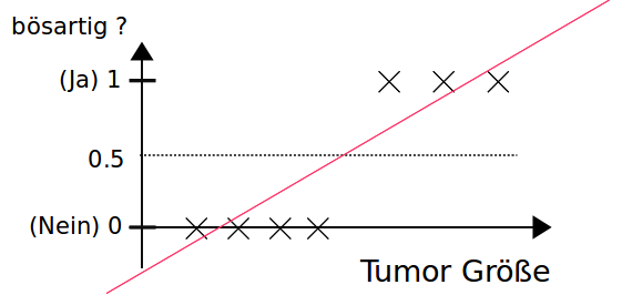
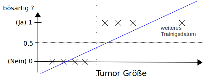
Using linear regression with a threshold for classification don't work properly.

Also note:

$h_{\Theta}(\vec x)$ can be greater than 1 or smaller than 0.

Logistic function (sigmoid)¶

We are looking for a function to squash the output:

$$ 0 \leq g(z) \leq 1 $$

That holds for the logistic function (sigmoid):

$$ g(z) = \frac{1}{1 + \exp(-z)} $$

Note:

$$ \frac{1}{1 + \exp(0)} = \frac{1}{2} $$

Logistic Regression Hypothesis¶

$$ h_\theta(\vec x) = g(\vec \theta^T \vec x) $$

with the logistic Function $g(z)$:

$$ h_\theta(\vec x) = \frac{1}{1 + \exp(-\vec \theta^T \vec x)} $$

Name 'logistic regression'¶

• Name part “logistic”: due to the use of the logistic function.
• Name part “regression” has historical reasons. But, it's not regression. It's classification!

Interpretation as probability¶

Discriminative model:

$$ h_\theta(\vec x) = p(y=1 \mid {\vec x}, \theta) $$

Conditional probability of $y=1$ under the constraint ${\vec x}$ and parameters $\theta$.

e.g. $ h_\theta({\vec x}) = 0.8$: probability for a malign tumor is 80%.

Prediction according to the probabilities. Usually: \begin{align} h\theta({\vec x}) & \geq 0.5 \rightarrow y=1 \ h\theta({\vec x}) & < 0.5 \rightarrow y=0 \end{align}

Decision Boundary¶

Decision boundary by thesholding¶

with threshold value 0.5 we have:

\begin{align} \vec \theta^T \cdot \vec x & \geq 0 \Rightarrow h\theta({\bf x}) \geq 0.5 \Rightarrow y{predicted}=1 \ \vec \theta^T \cdot \vec x & < 0 \Rightarrow h\theta({\bf x}) < 0.5 \Rightarrow y{predicted}=0 \end{align}

Example 1: $$ \vec \theta^T \vec x = \theta_0 + \theta_1 x_1 = -6. + \frac{6}{5} x_1 $$

Decision Boundary: $\vec \theta^T \vec x = 0 $

$\Rightarrow x_1 = 5$

Prediction:

• $x_1 \geq 5 \Rightarrow y_{predict} = 1$
• $x_1 < 5 \Rightarrow y_{predict} = 0$

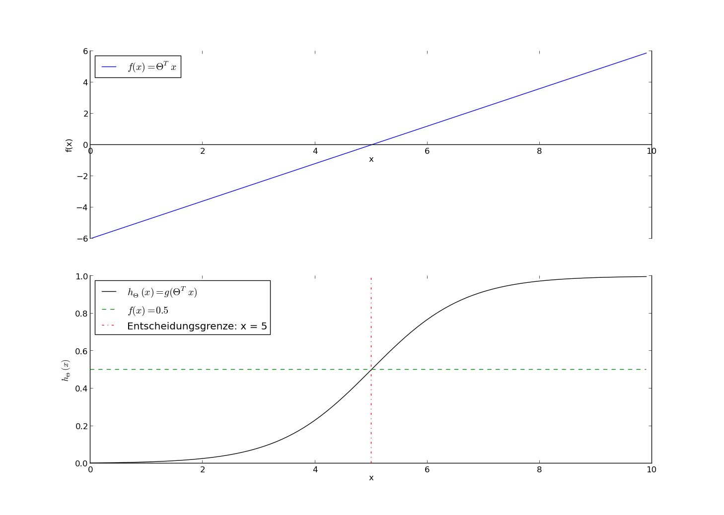
Example 2:

$$ \vec \theta^T \vec x = \theta_0 + \theta_1 x_1 + \theta_2 x_2 = 3 - x_1 - x_2 $$

Decision boundary:

$\vec \theta^T \vec x = 0 $ $\Rightarrow x_2 = 3 - x_1$

Prediction:

• $x_1 + x_2 \geq 3 \Rightarrow y_{predict} = 1$
• $x_1 + x_2 < 3 \Rightarrow y_{predict} = 0$

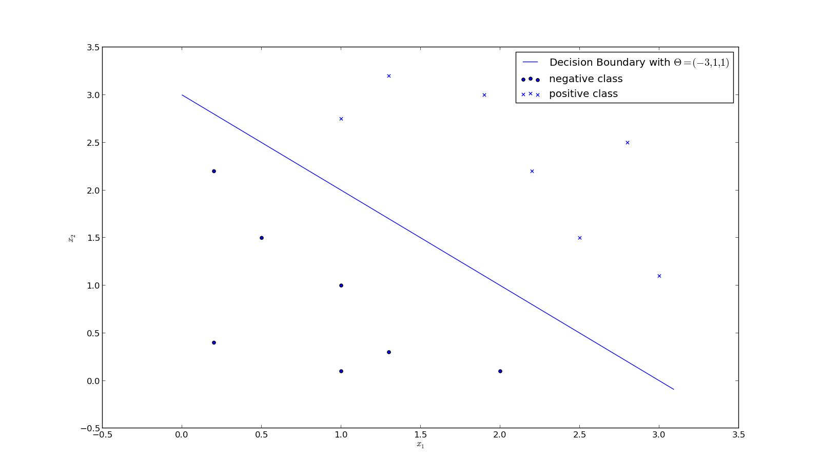
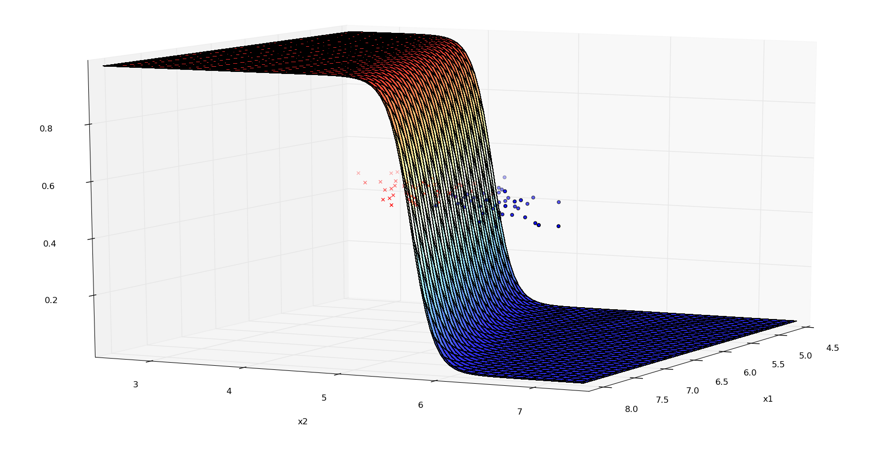
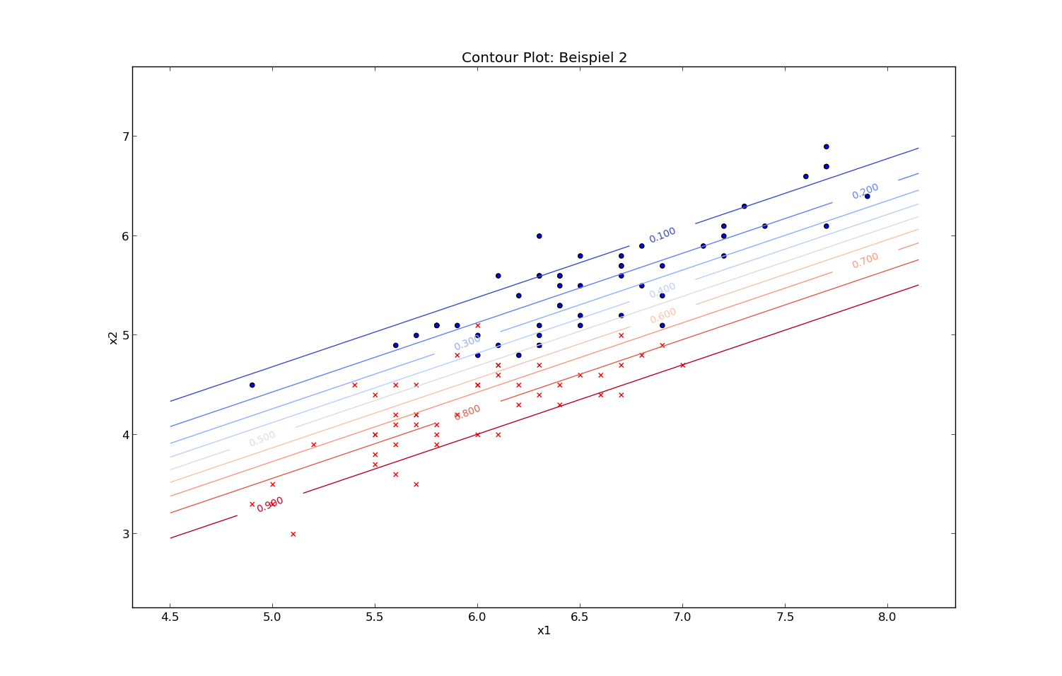
Example: Iris data set (just 2 classed and two features)

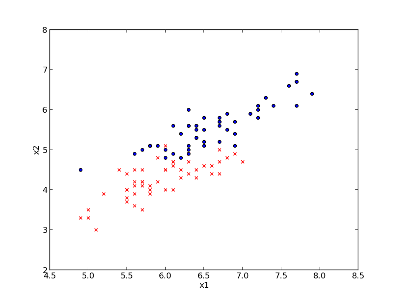
Classes: Iris-Versicolour (red), Iris-Virginica (blue)
Features: $x_1$: sepal length (cm) \hspace {1.5cm} $x_2$: petal length (cm)

Probabilities (3d-plot) - Iris data:

Probabilities (2d-plot) - Iris data:

Linear Separability¶

If we can separate the data points in n-dimensional space of two classes with a n-1 dimensional hyper plane than the classification problem is linearly separable.

Note: A hyper plane is formally defined by $\vec w^T \cdot \vec x = C$. So by definition logistic regression can solve only linearly separable data points completely ($C=-\theta_0$ and $w=(\theta_1, \dots, \theta_n)$).

Example: non linear separable data¶

Any ideas, how we can extend the model?

Non-linear basis functions $\phi({\bf x})$¶

Equation of a circle: $x_1^2 + x_2^2 = 1$}

Basis functions:

• $\phi_1({\bf x}) = x_1^2$
• $\phi_2({\bf x}) = x_2^2$

$$ h_\theta({\bf x})= g(\theta_0 + \theta_1 \phi_1({\bf x}) + \theta_2 \phi_2({\bf x}) ) $$$$ h_\theta({\bf x})= g(-1 + x_1^2 + x_2^2) $$

In the new feature space $\phi$ the data is linear separable:

With proper basis function we can solve complex problem.

Cost function for classification¶

Recap: Problem formulation¶

• Train data $\mathcal{D}$: $\{ ({\vec x}^{(1)},y^{(1)}), ({\vec x}^{(2)},y^{(2)}), \dots ({\vec x}^{(m)},y^{(m)\ }) \}$
  • ${\vec x}^{(i)} \in \mathbb{R}^{n+1}$, aa row vector $({\vec x}^{(i)})^T = (x_0,x_1, \dots, x_n)$ mit $x_0 =\ 1$
  • $y \in \{0,1\} $
• Hypothesis: $h_{\theta}(x) = 1 / (1 + \exp\{- \vec \theta^T {\vec x}\})$
• We are looking for "good" parameters $\theta$

Loss¶

Recap: cost for linear regression $$ J(\theta) = \frac{1}{2m} \sum_{i=1}^m (h_\theta({\vec x}^{(i)})-y^{(i)})^2 $$

Loss (pointwise cost for a training example):

$$ J(\theta) = \frac{1}{m} \sum_{i=1}^m loss(h_\theta({\vec x}^{(i)}),y^{(i)}) $$

squared loss function (for linear regression):

$$ \text{loss}(h_\theta({\vec x}),y) = \frac{1}{2} (h_\theta({\vec x})-y)^2 $$

Loss for logistic regression¶

• quadratic loss (squared loss) is not used for logistic regression
  • no convex problem
• from theorie ("maximum likelihood principle" ) we get another loss function.

Loss for an example of the positive class (y=1)¶

$\text{loss}(h_\theta(x^{(i)}), y^{(i)}) = -\log(h_\theta(x^{(i)}))$

Loss for an example of the negative class (y=o)¶

$\text{loss}(h_\theta(x^{(i)}), y^{(i)}) = 1-\log(1- h_\theta(x^{(i)}))$

Cross entropy¶

$$ \text{loss}(h_\theta(x^{(i)}), y^{(i)}) = - y^{(i)} \log (h_\theta(x^{(i)})) - (1 - y^{(i)}) \log \left( 1- h_\theta(x^{(i)})\right) $$\begin{align*} J(\theta) & = \frac{1}{m} \sum_{i=1}^{m} \text{loss}(h_\theta(x^{(i)}), y^{(i)}) \\ & = - \frac{1}{m} \left[ \sum_{i=1}^{m} y^{(i)} \log h_\theta(x^{(i)}) + (1 - y^{(i)}) \log \left( 1- h_\theta(x^{(i)})\right) \right] \end{align*}

Gradient descent¶

Problem formulation¶

• Hypothesis: $h_{\theta}(x) = 1 / (1 + \exp\{- \theta^T {\vec x}\})$
• Cost function:

\begin{align*} J_{\mathcal D}(\theta) %& = \frac{1}{m} \sum_{i=1}^{m} loss(h_\theta(x^{(i)}), y^{(i)}) \\ & = - \frac{1}{m} \sum_{i=1}^{m} \left[ y^{(i)} \log h_\theta({\vec x}^{(i)}) + (1 - y^{(i)}) \log \left( 1- h_\Theta({\vec x}^{(i)})\right) \right] \end{align*}

Goal: "good" parameters $\theta$ for the hypothesis $h_\theta({\bf x})$ by $\text{minimize}_{\theta} J(\theta)$

Update Rule for all $\theta_j$ (gradient descent) $$ \theta_j^{old} \leftarrow \theta_j^{old} - \alpha \frac{\partial}{\partial \theta_j} J(\theta^{old}) $$

\begin{align*} \frac{\partial}{\partial \theta_j} & J(\theta) = \\ \frac{\partial}{\partial \theta_j} & \left( - \frac{1}{m} \sum_{i=1}^{m} \left[ y^{(i)} \log h_\theta({\vec x}^{(i)})\ + (1 - y^{(i)}) \log \left( 1- h_\theta({\vec x}^{(i)})\right) \right] \right) = \\ & \dots = \frac{1}{m} \sum_{i=1}^{m} \left( h_\theta({\vec x}^{(i)})- y^{(i)}\right) x_j^{(i)} \end{align*}

So we get for the Update Rule:

$$ \theta_j^{new} \leftarrow \theta_j^{old} - \alpha \frac{1}{m} \sum_{i=1}^{m} \left( h_\theta({\vec x}^{(i)})- y^{(i)} \right) x_j^{(i)} $$

Exercise: Implementation of logistic regression¶

Note: Modify your "multivariate linear regression code", that your implementation works for linear and logistic regression.

1. Implement the logistic regression model as python function:

   get_logistic_hypothesis(theta)
   

   The python function should return a function, e.g.

   >> theta = np.array([1.1, 2.0, -.9]) 
   >> h = get_logistic_hypothesis(theta) 
   >> print h(X) 
   array([ -0.89896965,  0.71147926, ....

2. Implement (as function)

   1. the cross-entropy loss for logistic regression (in general for classification) and
   2. the squared-loss for linear regression.

   The function should return a function, e.g.

   >> loss = get_cross_entropy_loss(h, X, y)
   >> print loss(theta)
   array([ 7.3,  9.5, ....
   

   The array has m elements (number of data examples, i.e. a loss value for each example)
   Note: if we pass as argument h the function could be used for any classification problem (resp. regression problem.)

3. Implement the cost function:

   >> cost_function = get_cost_function(loss)
   

   loss and cost_function are functions with argument theta.

   >> cost_function(theta)
   15525.3

4. Implement gradient descent by using the functions above.

   1. Implement (modify) a function which does the update rule for computation of the new $\theta$ values:

      theta = compute_new_theta(x, y, theta, alpha, hypothesis)

   2. Implement (or modify) a function gradient_descent(alpha, theta, X, y). theta are the start values for $\vec \theta$. The function applies iteratively compute_new_theta. Use an arbitrary stoping criterion.

5. Use the artifical data (see below) for learning a logistic regression model. Plot the progress (cost value over iterations).

6. Plot the decision boundary together with the data scatter plot.
   Hint: $\theta_0 + \theta_1 x_1 + \theta_2 x_2 = 0$

7. Implement the computation of the classification error (one-line in numpy, no python loop!).
   classification error = number of wrong classified examples / number examples

Multiclass problems¶

Multiclass problems¶

by using binary classifier:

• One vs. All (One vs. Rest):

  • Train $k$ binary classifier $h^{(u)}$ for each class $u$.
  • Classification by $h = max_u h^{(u)}(x)$

• All vs. All (One vs. One or All-Pairs):

  • Train $k(k-1)$ binary classifier $h^{(uv)}$ for each pair of the classes $u$ and $v$ (Note $h^{(uv)}=h^{(vu)}$).
  • Classification by $h = max_u \sum_v h^{(uv)}(x)$

Softmax¶

• One-hot output encoding

  • for each class $i$ one Output $y_j$ with the target value
    • $y_j = 1$, if the train example belongs to class $j$
    • $y_j = 0$, else
  • for each class $k$ a parameter vector $\vec{\theta}_{k}$ (e.g. as matrix)

• Prediction of the probability that a data set with input vector $\vec{x}$ belongs to class k: $$ P(y=k \mid \vec x, \vec \theta_{k}) = softmax(\vec \theta_k \cdot \vec x) = \frac{e^{\vec \theta_k \cdot \vec x}}{\sum_j e^{\vec \theta_j \cdot \vec x}} $$

• Class prediction by $$ y_{pred} = argmax_k P(y=k \mid {\vec x}, \theta^{(k)}) $$

Literature¶

• Andrew Ng: Machine Learning. Openclassroom Stanford University, 2013
• C. Bishop: Pattern recognition and Machine Learning, Springer Verlag 2006
• Video: Nando de Freitas: Machine Learning, Logistic Regression
• M. Mohri et.al.: Foundation of machine learning, 2012