Learning Objectives
Concepts of machine learning
- Target function
- Overfitting, underfitting
- Generalization
- Out-of-sample error and test data
- Model complexity
Target function and noise
For prediction: We want to approximate an unknown function, the target function $t(\vec x)$.
If the targets $y$ would be deterministically determined from the $\vec x$ values:
$$ y = t(\vec {x}) $$
But $y$ is typically noisy. We can model this by:
$$ y^{(i)} = t(\vec {x}^{(i)}) + \epsilon $$
with a random variable $\epsilon$ (= stochastic noise)
Sidenote:
Instead of a function we now a a (conditional) probability distribution: $$ p(y \mid \vec {x}) $$
The probability distribution of the noise can depend on $\vec {x}$: $p(\epsilon \mid \vec {x})$.
Goal:
We are looking for "good" hypotheses. $$ h(\vec x) \approx t(\vec x) $$ for all $\vec{x}$ of interest, i.e. for all possible $\vec{x}$ we want to predict. ($p(\vec x)$ suffient large).
Training data is noisy: $y^{(i)} = t(\vec {x}^{(i)}) + \epsilon $
Therefore $h(\vec{x}^{(i)})$ should not perfectly match $y^{(i)}$ of the training data.
But how good should be the correspondence?
Sampling Error
- Which pattern are caused by the target function?
- Which pattern are caused by the (random chosen) train data?
Overfitting and Underfitting
import numpy as np
import matplotlib.pyplot as plt
%matplotlib inline
import numpy as np

def test_func(f, x, err=1.):
    return np.random.normal(f(x), err)

def compute_error(x, y, p):
    yfit = np.polyval(p, x)
    return np.sqrt(np.mean((y - yfit) ** 2))


def plot_under_overfit_polynoms():
    N = 10
    np.random.seed(45)
    x = np.linspace(-4, 3., N)
    quadratic_func = lambda x: -2 + 3. * x + -2. * x**2
    y = test_func(quadratic_func,x, 4.)

    xfit = np.linspace(-4, 3., 1000)

    degrees = [1, 2, 9]
    titles = ['d = 1 (under-fit)', 'd = 2', 'd = '+ str(degrees[2]) + ' (over-fit)']


    plt.figure(figsize = (9, 3.5))
    plt.subplots_adjust(left = 0.06, right=0.98,
                   bottom=0.15, top=0.85,
                   wspace=0.05)
    yticks = [-50,-40,-30,-20,-10, 0, 10]
    for i, d in enumerate(degrees):
        plt.subplot(131 + i, yticks=yticks)
        yticks=[]
        plt.scatter(x, y, marker='x', c='k', s=50)

        p = np.polyfit(x, y, d)
        yfit = np.polyval(p, xfit)
        plt.plot(xfit, yfit, '-b')

        #pl.xlim(-0.2, 1.2)
        plt.ylim(-55, 15)
        plt.xlabel(u'x')
        if i == 0:
            plt.ylabel('y')
        plt.title(titles[i])
Example: Linear Regression with polynominal basis functions
plot_under_overfit_polynoms()

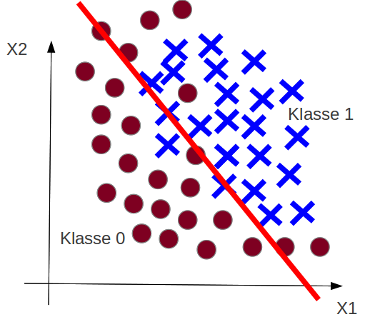
Example: Classification Underfitting
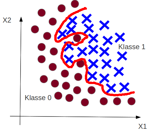
Example: Classification Overfitting
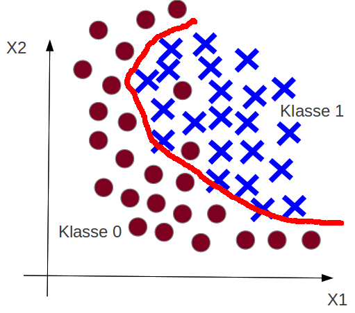
Example: Just Right
Goal of learning - Hypothesis Set $\mathcal{H}$}
Goal of learning: We are looking for a appropriate hypothesis $$ h(\vec x) \approx t(\vec x) $$
$h$ is determined from the hypothesis set $\mathcal{H}$ by training.
Example ``Univariate Linear Regression'':
$\mathcal H$ is the set of all (infinit) hypotheses: $h_\theta(x) = \theta_0 + \theta_1 x$ (by variation of $\theta_0$ and $\theta_1$).
From the set $\mathcal{H}$ we get through training a $\theta$, i.e. a hypothesis $h_{\theta_{final}}({x})$.
$h_{\theta_{final}}({\bf x})$ is given by the minimum of the cost function:
$\forall \theta: J(\theta_{final}) \leq J(\theta)$
Underfitting
Recap: Goal is $h(\vec x) \approx t(\vec x)$.
What happens in the underfitting case?
The goal can not be reached: No hypothesis of $\mathcal{H}$ is similar enough to $t(\vec x)$.
The hypothesis set $\mathcal{H}$ has not suffient complexity.
Overfitting
Recap: Goal is $h(\vec x) \approx t(\vec x)$.
What happens in the overfitting case?
The trained hypothesis $h_{\theta_{final}}({x})$ is adaped to much on the training data: also on the noise pattern.
The hypothesis set $\mathcal{H}$ has to much complexity.
Test data
Training error
Up to now only a training set $\mathcal{D}_{train}$ and calculation of the average loss of the traing data (cost function):
Training error (in-sample error $E_{in}(h)$):
$$ E_{in}(h) = \frac{1}{m} \sum_{i=0}^{m} loss(h(\vec x^{(i)}), y^{(i)}) $$
Note: We consider $E_{in}(h)$ now as a function of possible hypotheses $h$. We want to compare different models.
The low training error is not suffient to judge a "good" model.
Overfitting!
$h(\vec x)$ can make bad predictions for $\vec x$ values not in the training set.
Bad generalization.
Out-of-sample error
The out-of-sample error is the average loss of typical (new) data ($p({\vec x}', y')$ suffient large):
$$ E_{out}(h) = \mathbb{E}_{\bf x,y}\left[loss(h({\vec x}), y)\right] = \int\limits_{\mathcal{X \times Y}} loss(h({\vec x}), y) dp({\vec x},y) $$
Generalization error
The generalization error of a hypothesis $h$ can defined as (after [Abu]):
$$ | E_{out}(h) - E_{in}(h)| $$
Test data
Problem: We can compute the out-of-sample error $E_{out}$ directly.
Take $m_{test}$ labeled test data $\mathcal{D}_{test}$ to check if $h(\vec x)$ predicts good values even for $\vec x$ values not used in training.
$$ \mathcal{D}_{test}= \{ ( {\vec {x'}}^{(0)}, {y'}^{(0)} ), ( {\vec {x'}}^{(1)}, {y'}^{(1)} ), \dots, ( {\vec {x'}}^{(m_{test})}, {y'}^{(m_{test})} ) \} $$
Test error
The test error is the average loss of the test data:
$$ testerror = \frac{1}{m'} \sum_{i=0}^{m_{test}} loss(h({\vec {x'}}^{(i)}), {y'}^{(i)}) $$
The test error is an approximation of the out-of-sample error $E_{out}(h)$:
$$
testerror \approx \mathbb{E}_{\mathcal{X,Y}}[loss(h({\bf x}), y)] = E_{out}(h)
$$
Model complexity, Capacity
informal:
The complexity of $\mathcal{H}$ describes how many compex functions the hypothesis set $\mathcal{H}$ can cover.
Measure of model complexity are
- VC-Dimension $d_{vc}$ (Vapnik–Chervonenkis Dimension)
- Rademacher complexity
Expectation of out-of-sample error
Starting point for the Bias-Variance Analysis is the expectation of out-of-sample error:
$$ \mathbb{E}_{\mathcal{D}} \left[ E_{out}(h^{\mathcal{D}}({\bf x})) \right] $$
with
- $h^{\mathcal{D}}$: trained hypothesis from $\mathcal{D}$ (training data)
- $E_{out}(h^{\mathcal{D}})$: out-of-sample error for the trained hypothesis
- $\mathbb{E}_{\mathcal{D}}$: Expectation with respect to the training data (a training set is an event).
Bias-variance analysis
without noise and squared error: \begin{align*} \mathbb{E}_{\mathcal{D}} \left[ E_{out}(h^{\mathcal{D}}) \right] & = \mathbb{E}_{\mathcal{D}} \left[ \mathbb{E}_{\bf x,y} \left[ \left(h^{\mathcal{D}}({\bf x}) - t({\bf x})\right)^2 \right] \right] \\ & = \mathbb{E}_{\bf x,y} \left[ \mathbb{E}_{\mathcal{D}} \left[ \left(h^{\mathcal{D}}({\bf x}) - t({\bf x})\right)^2 \right] \right] \end{align*}
with the average hypothesis $$ \tilde{h}({\bf x}) = \mathbb{E}_{\mathcal{D}}\left[ h^{\mathcal{D}}({\bf x}) \right] $$
We get (see e.g. [Abu] p.63): \begin{align*} \mathbb{E}_{\mathcal{D}} \left[ E_{out}(h^{\mathcal{D}}({\bf x})) \right] &= \mathbb{E}_{\bf x,y} \left[ \mathbb{E}_{\mathcal{D}} \left[\left(h^{\mathcal{D}}({\bf x}) - \tilde{h}({\bf x}) \right)^2\right]\right] &+&\mathbb{E}_{\bf x,y} \left[ \left(\tilde{h}({\bf x}) -t({\bf x}) \right)^2 \right]& \\ &= variance &+&bias^2 \end{align*}
with noisy data there is a thrid term: the irreducable error $\mathbb{E}_{\mathcal X}[\epsilon^2]$ (Bayes Error, see e.g. [Has])}
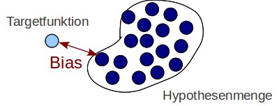
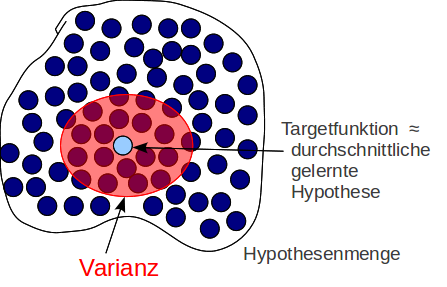
Interpretation: Bias
$$ \mathbb{E}_{\bf x,y} \left[ \left(\tilde{h}({\bf x}) -t({\bf x}) \right)^2 \right] $$ Quadratic deviation of the average hypothesis $\tilde h$ from the target function $t$ $\leftrightarrow$ Underfitting
Interpretation: Variance
$$ \mathbb{E}_{\bf x,y} \left[ \mathbb{E}_{\mathcal{D}} \left[\left(h^{\mathcal{D}}({\bf x}) - \tilde{h}({\bf x}) \right)^2\right]\right] $$
Average quadratic deviation {$h^{\mathcal{D}}$} from the average hyposesis $\tilde h$ $\leftrightarrow$ Overfitting
Example
from [Abu]
- Target function $sin(x)$
- $p(x)$: Uniform distributed in the range $(0, 2 \pi)$
- no noise
- only two training examples. i.e. $n=2$
- Model 1: $h(x)=w$ (constant)
- Model 2: $h(x)=\theta_0 + \theta_1 x$
Exercise
Approximate: $\mathbb E (E_{out})$, the bias and the variance for both models by sampling. A sample correspond to a training set (with 2 examples)
x, y  = train_data()
theta_0, theta_1 = get_theta(x, y)
plt.plot(x_, y_, 'b-')
plt.scatter(x,y,color='r')
plt.plot(x_,  theta_0 + theta_1 * x_, 'g-')

No noise on $y$ : $$ \mathbb E_{\bf x, \bf y} [ E_{out} ] = \int_{-\infty}^{\infty} (t(x)- h(x))^2 p(x) dx = \int_{0}^{2 \pi} (t(x)- h(x))^2 dx $$
expectation_Eout_1 = e_out_m1.mean()
print ("expectation of E_out of model 1:", expectation_Eout_1)
expectation_Eout_2 = e_out_m2.mean()
print ("expectation of E_out of model 2:", expectation_Eout_2)
# Average Model 1 and 2
plt.plot(x_, y_, 'b-', label='target function')
plt.plot(x_,  avg_theta_0 + avg_theta_1 * x_, 'r-', label='average model 2')
plt.plot(x_,  np.ones(len(x_)) * avg_w, 'g-', label='average model 1')
plt.xlabel("x"); plt.ylabel("y"), plt.legend()

From the plot we see that the bias of model 2 is smaller than the bias of model 1.
print ("Bias of model 1:", bias_1)
print ("Bias of model 2:", bias_2)
print ("Variance of model 1:", variance_1)
print ("Variance of model 2:", variance_2)
print("model 1: E_out ≈ bias + variance:  %f ≈ %f + %f" % (expectation_Eout_1, bias_1, variance_1))
print("model 2: E_out ≈ bias + variance:  %f ≈ %f + %f" % (expectation_Eout_2, bias_2, variance_2))
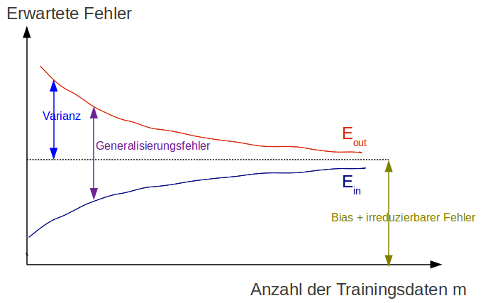
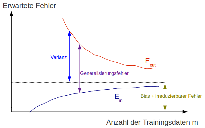
Learning curves
Goal
$$ h(\vec x) \approx t(\vec x) $$ reached if $E_{out}$ is small (small test error)
Both conditions must be satisfied
- $E_{in}$ small training error (low bias, no underfitting)
- Small generalization error $|E_{out} -E_{in}|$ respectively $test error \approx trainings error$ (low variance, no overfitting)
How can we know that the model is adequate?
Adequate in respect to:
- Number of training data $m$ of $\mathcal{D}_{train}$
- Model complexity $\mathcal{H}$
- Signal-noise ration: strength of stochastic noise $\epsilon$ in respect to the target function $t$
Learning curve of a simple model
Learning curve of a complex model
Literature:
- [Abu] Yaser Abu-Mostafa
- Learning from Data, Caltech Machine Learning
- Learning from Data, AMLBook 2012
- Andrew Ng: Machine Learning. Openclassroom Stanford University, 2013
- [Has] Trevor Hastie,Robert Tibshirani, Jerome Friedman: The Elements of Statistical Learning, Chaper 7, Springer Verlag 2009